This year, I participated in the Hermannslauf, a public run from Detmold to Bielefeld. Since then, I wanted to have a look at the results in more detail.
The data can be found here. My tool of choice is R, a programming language for statistical analyses and data visualisation. I am using tidyverse packages (more information about the tidyverse can be found on its homepage http://tidyverse.org) for the analysis, a collection of packages designed to work together.
How to get the data
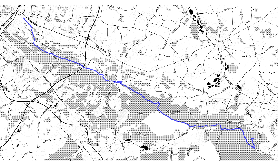
During the run, I tracked the route with Meerun.
The resulting .gpx file can be loaded and processed with R.
I used import functions I wrote for a different project (more on this topic in a future article) to load and plot the track.
The results can be retrieved as .json elements.
I will not go into detail about the retrieval today but rather focus on the analysis.
url <- "http://www.davengo.com/event/result/45-hermannslauf-2016/search/list"
start_offset <- 0
end_offset <- 5625
all_data <- tibble::data_frame()
for (i in seq(start_offset, end_offset, 125)) {
    body <- list(
        type = "simple",
        term = NULL,
        category = "31,1 km Hermannslauf",
        offset = i
        )
    response <- httr::POST(url, body = body, encode = "json")
    httr::stop_for_status(response)
    raw_data <- httr::content(response)
    raw_data <- raw_data$results
    if (length(raw_data) == 0) {
        writeLines(c("Stopped at i = ", i), sep = "")
        return(all_data)
    }
    all_data <- c(all_data, list(raw_data))
    }
The data are now buried in a list of lists of lists and can be processed further.
Data tidying
After all the data are retrieved, it is easy to unwrap the present and have a peek at the content:
df <- flatten(raw_data) %>%
bind_rows() %>%
select(-hash, -combined) %>%
mutate(Gender = if_else(is.na(rankFemale), "m", "f")) %>%
select(-rankFemale, -rankMale)
names(df) <- c("Team", "Number", "Name", "Age", "Rank", "Time", "First_name", "Rank_age_group", "Gender")
df$Time <- as.POSIXct(df$Time, format = "%H:%M:%S", origin = "2016-04-30")
df$Age <- as.factor(df$Age)
levels(df$Age) <- c(30, 35, 40, 45, 50, 55, 60, 65, 70, 75, 80, "H", "J", 30, 35, 40, 45, 50, 55, 60, 65, 70, 75, "H", "J")
df$Age <- factor(df$Age, levels = c("J", "H", "30", "35", "40", "45", "50", "55", "60", "65", "70", "75", "80"), ordered = TRUE)
df <- select(df, Name, First_name, Time, Rank, Rank_age_group, Age, Gender, Number, Team)
df
This is our data frame with which I will be answering all my questions:
## # A tibble: 5,723 × 9
##         Name First_name                Time  Rank Rank_age_group   Age
##        <chr>      <chr>              <dttm> <int>          <int> <ord>
## 1       Name      Name 2016-11-12 01:49:10     1              1    35
## 2       Name      Name 2016-11-12 01:51:02     2              1     H
## 3       Name      Name 2016-11-12 01:52:09     3              2    35
## 4       Name      Name 2016-11-12 01:52:30     4              3    35
## 5       Name      Name 2016-11-12 01:52:40     5              2     H
## 6       Name      Name 2016-11-12 01:55:42     6              3     H
## 7       Name      Name 2016-11-12 01:56:04     7              4     H
## 8       Name      Name 2016-11-12 01:56:32     8              1    45
## 9       Name      Name 2016-11-12 01:56:35     9              5     H
## 10      Name      Name 2016-11-12 01:56:51    10              2    45
## # ... with 5,713 more rows, and 3 more variables: Gender <chr>,
## #   Number <int>, Team <chr>
The age groups H and J stand for Haupt and Jugend and probably contain ages 20 – 24 and 25 – 29, respectively. All the other age groups represent an age range of five years, e.g. the group 30 contains runners from 30 to 34 years.
Analysis
My results
Now, that all the data are in one tidy data frame the analysis can begin. First, let’s look at my results. How well did I fare? For all the questions the tidy data frame can be »queried«.
df %>% filter(Name == "Rüßler")## # A tibble: 1 × 9
## Name First_name Time Rank Rank_age_group Age Gender
## <chr> <chr> <dttm> <int> <int> <ord> <chr>
## 1 Rüßler Martin 2016-11-12 03:05:07 2906 367 30 m
## # ... with 2 more variables: Number <int>, Team <chr>So, I am on rank 2906 of 5723. Not too bad for my first run, I think.
All results
How does it compare to the others?
ggplot(data = df, aes(x = Time, colour = Gender, fill = Gender)) +
annotate("text", x = median(df$Time), y = 105, label = "Median") +
geom_segment(aes(x = median(df$Time), y = 0, xend = median(df$Time), yend = 100), colour = "black") +
geom_histogram(binwidth = 60) +
labs(title = "Distribution of running time", x = "Time", y = "Count")
Almost exactly median time!
Percentage of women
We can also see that far more men than women participated in the run. How many exactly?
df %>% group_by(Gender) %>%
summarise(Count = n())
## # A tibble: 2 × 2
## Gender Count
## <chr> <int>
## 1 f 1212
## 2 m 4511Age
What about the age distribution? What ages are participating the most?
df %>% group_by(Age, Gender) %>%
summarise(Count = n()) %>%
ggplot(aes(x = Age, y = Count)) +
geom_bar(aes(fill = Gender), stat = "identity", position = "dodge") +
labs(title = "Distribution of age")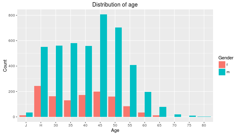
This graph draws a highly different picture for men and women. While the biggest group of female runners is the Haupt group, men between 45 and 54 are most frequent among the male runners. Is the midlife crisis driving men to participate in athleticism?
Number
Another question I was asking myself is whether the number is an indicator of the individual’s finishing place, i.e. whether the fastest runners also enrol earlier for the Hermannslauf than others. This assumes, of course, that the number is assigned in order of enrolment. First, a plot of number versus time to get an impression of the data.
df %>% group_by(Gender) %>%
ggplot(aes(x = Number, y = Time)) +
geom_point(size = 0.5) +
geom_smooth() +
labs(title = "Running time vs. number", x = "Number", y = "Time")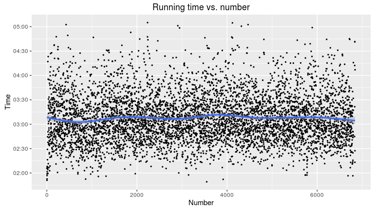
The package Intubate provides standard R functions with pipe support.
In this case, I can use lm.
library(broom)
library(intubate)
df %>% ntbt_lm(Number ~ Rank) %>%
tidy()
## term estimate std.error statistic p.value
## 1 (Intercept) 3.314367e+03 51.79919801 63.984901 0.00000000
## 2 Rank 3.107841e-02 0.01567484 1.982694 0.04744936Apparently, there is no correlation between the number and final rank. But there is a small cluster right at the beginning. A closer look reveals that this group of men were really fast in both regards, running and enrolment:
df %>% filter(Number <= 15, Gender == "m") %>%
ggplot(aes(x = Number, y = Time)) +
geom_point(size = 0.5) +
geom_smooth(method = "lm") +
labs(title = "Running time vs. number (detail)")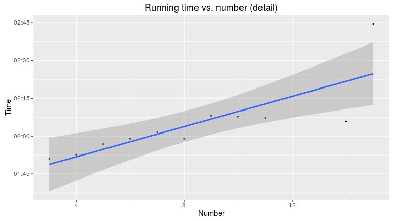
df %>% filter(Number <= 15, Gender == "m") %>%
ntbt_lm(Number ~ Rank) %>%
tidy()
## term estimate std.error statistic p.value
## 1 (Intercept) 7.476406711 1.068633924 6.996228 6.351134e-05
## 2 Rank 0.006382947 0.002837795 2.249263 5.106469e-02Most of these runners from the cluster are members of the TSVE 1890 Bielefeld, which organised the run.
Teams
I was also interested in the teams. How many runners run without a team? And what are the biggest teams?
df %>% group_by(Team, Gender) %>%
summarise(Count = n()) %>%
arrange(desc(Count))
## Source: local data frame [1,369 x 3]
## Groups: Team [1,161]
##
## Team Gender Count
## <chr> <chr> <int>
## 1 m 2161
## 2 f 521
## 3 TSVE 1890 Bielefeld m 149
## 4 LG Oerlinghausen m 68
## 5 TSVE 1890 Bielefeld f 67
## 6 Laufspass SW Sende m 60
## 7 Laufspass SW Sende f 42
## 8 CLAAS m 30
## 9 Active Sportshop Herford f 27
## 10 Active Sportshop Herford m 26
## # ... with 1,359 more rows2161 of 4511 men (roughly 48 %) and 521 of 1212 women (roughly 43 %) had no team affiliation. Those can be excluded with a filter to create a list containing the number of runners per team. Here, the results are not grouped by gender. I am only showing the first ten results:
df %>% group_by(Team) %>%
summarise(Team_Size = n()) %>%
arrange(desc(Team_Size)) %>%
filter(Team != "") %>%
head(n = 10)
## # A tibble: 10 × 2
## Team Team_Size
## <chr> <int>
## 1 TSVE 1890 Bielefeld 216
## 2 Laufspass SW Sende 102
## 3 LG Oerlinghausen 94
## 4 Active Sportshop Herford 53
## 5 LC Solbad Ravensberg 38
## 6 Non-Stop-Ultra 35
## 7 CLAAS 32
## 8 Teuto Runner 30
## 9 LV Oelde 26
## 10 uniRenner 26Look, there’s my team, the uniRenner! We and LV Oelde share rank 9. The TSVE 1890 Bielefeld as the organiser of the Hermannslauf is by far the largest team and its many members are actively participating in the run. This is visualised in the following bar chart:
df %>% group_by(Team) %>%
summarise(Count = n()) %>%
arrange(desc(Count)) %>%
filter(Team != "", Count <= 15) %>%
ggplot(aes(x = Count)) +
geom_bar() +
labs(title = "Team sizes", x = "Number of teams", y = "Team size")
How many teams are there in total?
df %>% group_by(Team) %>%
summarise(Team_Size = n()) %>%
arrange(desc(Team_Size)) %>%
filter(Team_Size == 1) %>%
nrow()
## [1] 738There are many teams with just one member. This may be due to spelling errors which I have not checked for.
I hope that I could show how relatively simple it is to do an exploratory data analysis and have fun with it as well. This is but a fraction of questions to analyse and I already have some new ideas which I will discuss in a future article.
Title image by David Marcu.