A few days ago I saw this tweet:
Dataset of Los Angeles water use by zip code. Would be interesting to see mapped! https://t.co/xQuoynCfMN #DataScience #OpenData pic.twitter.com/6pLEiRGJfq
— Cool Datasets (@CoolDatasets) January 3, 2017
This seemed to be a great opportunity to work with spatial data! I have been experimenting with geographical data before, so I thought that this could be a manageable task. Two kinds of data are needed here:
- The data mentioned in the tweet, and
- spatial data about the ZIP codes.
Preparing the water data
The data set can be found on Datazar and contains 119 observations of 9 variables. Of course, the data format does not adhere to the rules of tidy data. Let’s try and change that. In addition to the tidyverse package bundle, I will be using a few more packages which are either tidyverse packages not loaded by default or required for spatial analyses.
library(magrittr)      # To access the »boomerang« pipe %<>%
library(tidyverse)     #
library(rgdal)         # For loading spatial data
library(broom)         #
library(ggmap)         #
library(gganimate)     # Make a nice animation
library(RColorBrewer)  # Adjustment of the colour palette

water <- read_csv("~/src/la-water/data/Los_Angeles_Water_Use_Average_By_Zipcode.csv",
         col_types = "iiiiiiiic")
water
# A tibble: 119 × 9
   `FY 05/06` `FY 06/07` `FY 07/08` `FY 08/09` `FY 09/10` `FY 10/11` `FY 11/12` `FY 12/13`
        <int>      <int>      <int>      <int>      <int>      <int>      <int>      <int>
1          32         36         34         32         27         26         36         16
2          18         19         17         14         13         13         13         12
3          62         66         58         65         55         52         44         36
4          31         35         32         31         26         26         27         24
5          47         52         50         49         41         41         44         26
6          23         26         24         23         17         16         18         18
7          98         99         93         90         84         82         82         37
8          28         27         26         25         20         21         23         10
9         117        119        107        106        101        102        101          8
10         16         17         16         15         15         14         14         10
# ... with 109 more rows, and 1 more variables: `Location 1` <chr>

water[,9]
# A tibble: 119 × 1
                                       `Location 1`
                                              <chr>
1   91342\n(34.30514302800049, -118.43521825999971)
2   91309\n(34.21867307400049, -118.59758676999968)
3    91302\n(34.14327419400047, -118.6628270279997)
4   90272\n(34.04886156900045, -118.53572692799969)
5    91316\n(34.16673287800046, -118.5162960619997)
6   91214\n(34.228570997000475, -118.2469491709997)
7   90020\n(34.06636325100044, -118.30164844599972)
8   90248\n(33.87544370900048, -118.28237834699968)
9  90012\n(34.059480762000476, -118.24204800599972)
10  90062\n(34.00387338200045, -118.30885680999972)
# ... with 109 more rows
We have information about water use from the fiscal years 05/06 up to 12⁄13. As we can see, the information about the year is only available as column names. There is no single variable containing the water usage data. The last variable even contains newline characters! We can use the gather function from the tidyr package to re-format the first part of the data. In order to have nicer values in the final data frame, the column names are best adjusted before the transformation. The location variable should be left unchanged, at least for now.
names(water) <- c("05/06",
                  "06/07",
                  "07/08",
                  "08/09",
                  "09/10",
                  "10/11",
                  "11/12",
                  "12/13",
                  "Location")

water %<>% gather(FY, Use, -Location, convert = TRUE)
water
# A tibble: 952 × 3
                                           Location    FY   Use
                                              <chr> <chr> <int>
1   91342\n(34.30514302800049, -118.43521825999971) 05/06    32
2   91309\n(34.21867307400049, -118.59758676999968) 05/06    18
3    91302\n(34.14327419400047, -118.6628270279997) 05/06    62
4   90272\n(34.04886156900045, -118.53572692799969) 05/06    31
5    91316\n(34.16673287800046, -118.5162960619997) 05/06    47
6   91214\n(34.228570997000475, -118.2469491709997) 05/06    23
7   90020\n(34.06636325100044, -118.30164844599972) 05/06    98
8   90248\n(33.87544370900048, -118.28237834699968) 05/06    28
9  90012\n(34.059480762000476, -118.24204800599972) 05/06   117
10  90062\n(34.00387338200045, -118.30885680999972) 05/06    16
# ... with 942 more rows
I have come to like what I call the »boomerang« pipe, %<>. It pipes the variable on the left side and assigns the result back to it. This makes short and clean code, in my opinion.
In a second step, we need to deconstruct the location variable and extract the ZIP code, longitude, and latitude information. Luckily, there already is a handy function for that, separate. It accepts Regular expressions which we can use to define the cutting positions. Basically, it cuts where there is no number, period, or minus sequence of length 1 or longer.
water %<>% separate(
  col = Location,
  into = c("Zip_Num", "Latitude", "Longitude"),
  sep = "[^[0-9.-]]+",
  extra = "drop",
  convert = TRUE) %>%
  group_by(FY)

water
Source: local data frame [952 x 5]
Groups: FY [8]

   Zip_Num Latitude Longitude    FY   Use
*    <int>    <dbl>     <dbl> <chr> <int>
1    91342 34.30514 -118.4352 05/06    32
2    91309 34.21867 -118.5976 05/06    18
3    91302 34.14327 -118.6628 05/06    62
4    90272 34.04886 -118.5357 05/06    31
5    91316 34.16673 -118.5163 05/06    47
6    91214 34.22857 -118.2469 05/06    23
7    90020 34.06636 -118.3016 05/06    98
8    90248 33.87544 -118.2824 05/06    28
9    90012 34.05948 -118.2420 05/06   117
10   90062 34.00387 -118.3089 05/06    16
# ... with 942 more rows
By the way: the units for water use are hundred cubic feet [HCF]. With the water data prepared, we can now move on to the spatial data.
Preparing the spatial data
Spatial data for the United States are readily available. I found a suitable data set on the Los Angeles County GIS Data Portal as well with a description of its features. Since the data will be used for plotting with ggplot2, a bit of transformation is needed here. First of all, the projection should match the one we are used to on maps: WGS84.
setwd("~/src/la-water/data/") # Adapt as necessary
ogrListLayers(".")
lashape <- readOGR(dsn = ".", layer = "CAMS_ZIPCODE_STREET_SPECIFIC")
lashape <- spTransform(lashape, CRS("+proj=longlat +datum=WGS84"))
lashape@data$id = rownames(lashape@data)
lazips <- lashape %>% tidy(region = "id") %>%
  left_join(y = lashape@data, by = "id")
lazips %<>% filter(Zip_Num %in% water$Zip_Num)
In the last pipe, all ZIP codes for which the water data set does not contain any information are filtered out. lazips contains information about the shapes and positions of the ZIP codes.
Merging both data sets
water$Zip_Num <- as.factor(water$Zip_Num)
lamerge <- inner_join(lazips, water, by = "Zip_Num")
Plotting
All the data are in place. Two data layers are used here:
- The ZIP code areas coloured according to water consumption, and
- The borders between these areas.
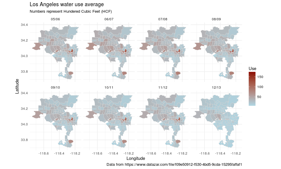
The rest mostly is cosmetics. In order to make change more prominent I chose a colour gradient from blue to red.
ggplot(lamerge, aes(long, lat, group = group)) +
  geom_polygon(aes(fill = Use)) +
  geom_path(colour = "lightgrey", size = .2) +
  scale_fill_gradient(low = "lightblue", high = "darkred") +
  facet_wrap( ~ FY, ncol = 4) +
  coord_equal() +
  theme_minimal() +
  labs(x = "Longitude", y = "Latitude", title = "Los Angeles water use average", subtitle = "Numbers represent Hundered Cubic Feet (HCF)", caption = "Data from https://www.datazar.com/file/f09e50912-f530-4bd5-9cda-15295faffaf1")
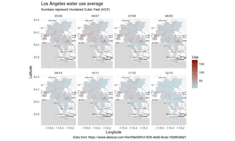
We can see that for the last fiscal year, 12 /13, the water consumption looks a lot more »blue« than for the previous years.
Adding a background map
For an easier orientation, the data can also be overlayed on a map. The only thing to do here is to save a map. For the rest, we can use the existing plotting commands from before.
# Map of Los Angeles by address
lamap <- get_map(location = "Los Angeles", source = "stamen", maptype = "toner-lite")

ggmap(lamap, extent = "device") +
  geom_polygon(aes(long, lat, group = group, fill = Use), alpha = 0.7, data = lamerge) +
  geom_path(aes(long, lat, group = group), colour = "lightgrey", size = 0.2, data = lamerge) +
  scale_fill_gradient(low = "lightblue", high = "darkred") +
  facet_wrap( ~ FY, ncol = 4) +
  labs(x = "Longitude", y = "Latitude", title = "Los Angeles water use average", subtitle = "Numbers represent Hundered Cubic Feet (HCF)", caption = "Data from https://www.datazar.com/file/f09e50912-f530-4bd5-9cda-15295faffaf1") +
  theme_minimal()
Creating an animation
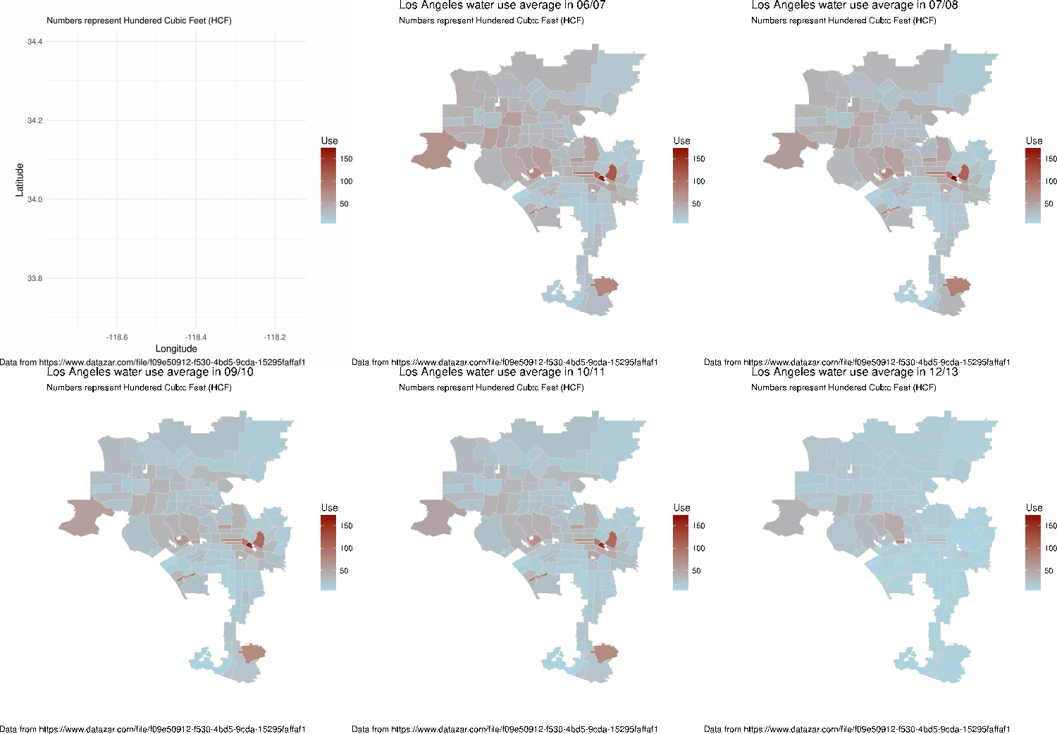
The changes would be better visible in an animation. With the help of the gganimate package only a single adjustment has to be made to the plot: the frame aesthetic. The animation can be exported to various formats.
water$Zip_Num <- as.factor(water$Zip_Num)
tmp <- left_join(lazips, water)

anim <- ggplot(lamerge, aes(long, lat, group = group, frame = FY)) +
  coord_equal() +
  geom_polygon(aes(long, lat, group = Zip_Num, fill = Use)) +
  geom_path(colour = "lightgrey", size = .2) +
  scale_fill_gradient(low = "lightblue", high = "darkred") +
  theme_minimal() +
  labs(x = "Longitude", y = "Latitude", title = "Los Angeles water use average in", subtitle = "Numbers represent Hundered Cubic Feet (HCF)", caption = "Data from https://www.datazar.com/file/f09e50912-f530-4bd5-9cda-15295faffaf1")
gganimate(anim, "la-water.gif")
I also put the code into a gist for easier copying. Feel free to play with it.
Cover image by Austin Lee.