Birth and Moon

Some time ago, before the birth of my second child, a colleague of mine told me they think that there is a connection between the moon and the possibility of giving birth and that I just had to look up the next full moon to know when the child is due.

Since I was not convinced right away, I chose to see for myself.

Hey moon, what’s up?

The first question I tried to solve was to get information about the moon phase. A simple web search for »R moon« brought up the package lunar. You can find a description in the manual on CRAN. When I played around with it I discovered that it had all I need for my project. For any date, the lunar phase could be calculated, as one of

a list of four (new, waxing, full, waning),
a list of eight (new, waxing crescent, first quarter, waxing gibbous, full, waning gibbous, last quarter, waning crescent), or
the moon phase in radians.

Show me the data

Now I only needed actual data to put my colleague’s assumption to the test. Luckily for me, there is something perfectly suited for my case. The U.S. Centers for Disease Control and Prevention (CDC) published a fitting data set which is also part of the Google BigQuery example data sets. That means I can directly access the data via another R package, bigrquery. Since the data set is too big to use in full, I also needed a way to get a sample.

Getting my hands dirty

The first step to do was the import of the data. To get a random sample from the huge data set I used the answer to a Stack Overflow question about random sampling in Google BigQuery.

set.seed("4711")

library(magrittr)
library(tidyverse)
library(bigrquery)
library(ggalt)
library(lubridate)

project_id <- "my-bigrquery"
query_lunar <- "SELECT year, month, day
                FROM [publicdata:samples.natality]
				WHERE year < 1989
				AND RAND() < 100000/137826763
				LIMIT 100000"
natality_raw <- query_exec(query_lunar, project = project_id, max_pages = Inf) %>%
  as_tibble()

As an output, the duration of the query’s execution was displayed:

Running job -:  3s:2.5 gigabytes processed

This left me with a table of 100k observations in the R workspace. The next step was data inspection and tidying. It is always useful to inspect the data before starting to work on it. The natality data, for example, changed insofar as that the day variable is omitted for all entries after 1989-01-01. Invalid or unknown days have the value “99”. This is the reason for the WHERE condition in the query. For a maximum of detail I chose to calculate the lunar phase in radians.

I wanted to remove invalid days, have a single date column, remove unnecessary columns, and add the lunar phase for each date before proceeding further.

natality_raw %>%
  filter(day < 32) %>%
  mutate(date = as.Date(paste(year, month, day, sep = "-"))) %>%
  select(-one_of(c("year", "month", "day"))) %>%
  select(date, everything()) %>%
  mutate(lunar_phase = as.numeric(lunar::lunar.phase(date)) - pi) %>%
  mutate_at(vars(lunar_phase), round, digits = 1) %>%
  group_by(lunar_phase) %>%
  summarise(n = n()) %>%
  na.omit() ->
  natality

natality
# A tibble: 63 x 2
lunar_phase     n
<dbl> <int>
1       -3.10   579
2       -3.00   642
3       -2.90   634
4       -2.80   642
5       -2.70   675
6       -2.60   663
7       -2.50   619
8       -2.40   645
9       -2.30   648
10      -2.20   664
# ... with 53 more rows

The result

Now I could visualise the cleaned data.

p <- ggplot(natality, aes(x = lunar_phase, y = n)) +
  geom_lollipop(point.colour = "orange", point.size = 2) +
  theme_minimal() +
  labs(title = "Distribution of births over lunar phase",
       x = "Lunar phase [rad]", y = "Number of births",
       caption = "Data from the natality data set")
p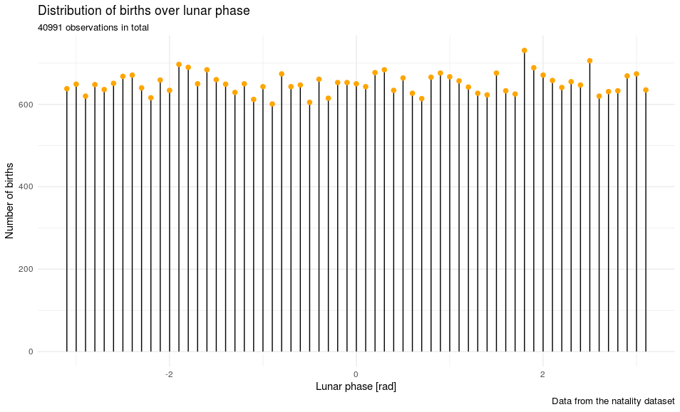

Distribution of births over lunar phase

It looks like the moon has no observable influence on the distribution of those births. Question answered.

…and beyond

But if I made so much effort to get here, I might as well have another look at the data. For example, are there other factors that influence the date of birth? How about the day of week?

# Create a column for day of week
natality_raw %>%
  filter(day < 32) %>%
  mutate(date = as.Date(paste(year, month, day, sep = "-"))) %>%
  select(-one_of(c("year", "month", "day"))) %>%
  select(date, everything()) %>%
  mutate(weekday = wday(date, week_start = 1, label = TRUE)) %>%
  group_by(weekday) %>%
  summarise(n = n()) %>%
  na.omit() ->
  natality

p <- ggplot(natality, aes(x = weekday, y = n)) +
  geom_lollipop(point.size = 2, aes(colour = colour), show.legend = FALSE) +
  theme_minimal() +
  labs(title = "Distribution of births over weekdays",
       subtitle = "40991 observations in total",
       x = "Day of week", y = "Number of births",
       caption = "Data from the natality data set")
p

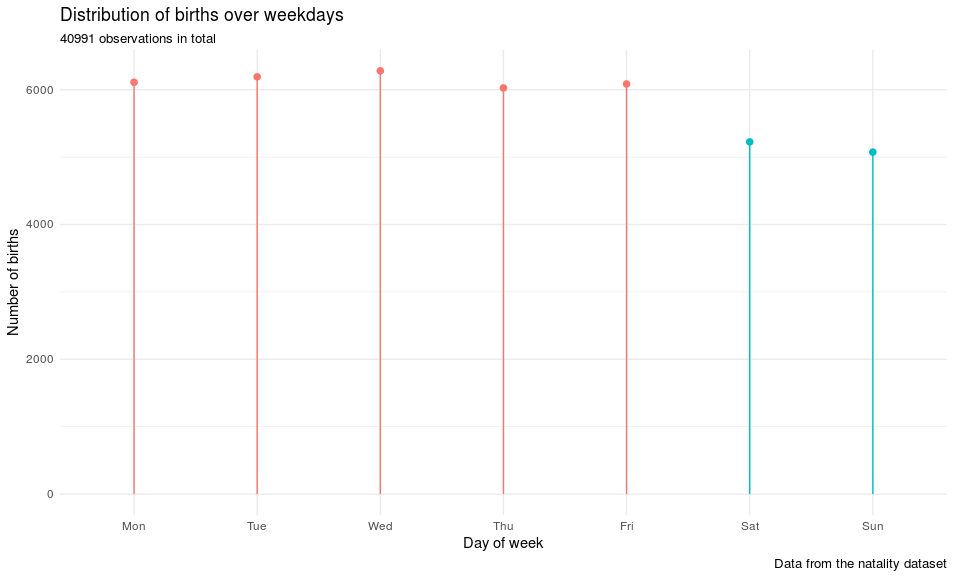
Distribution of births over weekdays

This looks like there is a lower rate of birth on the weekend. One reason for this might be that caesareans do not occur on weekends if there is no medical emergency. Unfortunately, the type of birth is not encoded in the data set.

What else can we look at? Seasonality comes to mind. More often than not I get the impression that the number of births peaks in September. Is this supported by the data?

natality_raw %>%
filter(day < 32) %>%
mutate(date = as.Date(paste(year, month, day, sep = "-"))) %>%
mutate(doy = as.integer(yday(date))) %>%
na.omit() %>%
mutate(weekday = wday(date, week_start = 1, label = TRUE)) %>%
group_by(doya) %>%
summarise(n = n()) -> natality

p <- ggplot(natality, aes(x = doy, y = n)) +
  geom_line() +
  theme_minimal() +
  geom_smooth(col = "orange") +
  labs(title = "Distribution of births over day of year",
	   subtitle = "40991 observations in total",
	   x = "Day of year", y = "Number of births",
	   caption = "Data from the natality data set")

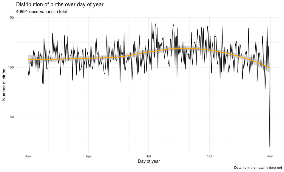
Distribution of births over day of the year

It looks like there is a slightly higher rate of birth in early autumn. There are many more things to look at (and also other people’s blog posts), but I will stop here and follow up on this article.

Cover image by Celso